io.github.mbk-dev/okama-mcp
Portfolio analytics via the okama library: backtests, Monte Carlo, efficient frontier, PNG charts
Open source Open in the app JSON README (API)
About
Portfolio analytics via the okama library: backtests, Monte Carlo, efficient frontier, PNG charts
Details
- Kind
- MCP servers
- Topic
- Finance & crypto
- Publisher
- mbk-dev
- Origin
- official
- Category
- ferramentas
- Transport
- local
- Version
- 1.9.0
- Stars
- 4
- Last push
- 2026-08-31T18:18:45Z
- Repository state
- ativo
- Language
- Python
- License
- MIT
- Added
- 2026-08-29 04:00:29
- Updated
- 2026-08-31 16:00:09
- Origin id
io.github.mbk-dev/okama-mcp
README
# okama-mcp
<!-- mcp-name: io.github.mbk-dev/okama-mcp -->
[](https://pypi.org/project/okama-mcp/)
[](https://github.com/mbk-dev/okama-mcp/actions/workflows/ci.yml)
[](https://pypi.org/project/okama-mcp/)
[](LICENSE)
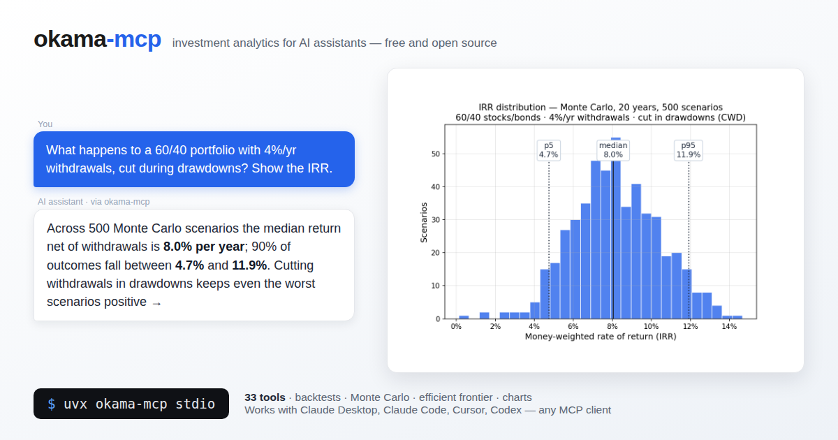
MCP (Model Context Protocol) server that exposes the [okama](https://github.com/mbk-dev/okama)
investment portfolio toolkit to AI assistants — Claude Desktop, Claude Code, Cursor, Codex,
and any other MCP-compatible client.
With okama-mcp installed, you can ask an AI things like:
> *"Backtest a portfolio of 30% gold and 70% real estate over the last 15 years."*
>
> *"Run a Monte Carlo retirement forecast on that portfolio, withdrawing $1,000/month
> indexed to inflation, over 25 years."*
>
> *"What's the tangency portfolio of SPY, BND, and GLD with a 3% risk-free rate?"*
…and the AI uses the MCP tools to call okama directly — no Python code needed.
Built on [FastMCP](https://github.com/jlowin/fastmcp). Single codebase, two transports:
`stdio` (for local clients) and `streamable-http` (for self-hosting).
okama-mcp is free and open source — no hosted service, no registration; you run it
yourself, locally or on your own server.
## Install
Requires Python ≥ 3.11 (same floor as okama itself); okama ≥ 2.2.0 is installed automatically.
The easiest way — no clone, no venv — is [uv](https://docs.astral.sh/uv/) or pipx:
```bash
uvx okama-mcp stdio # run straight from PyPI
# or
pipx install okama-mcp
```
Plain pip works too:
```bash
pip install okama-mcp
```
> [!WARNING]
> <sub>With pip, prefer a dedicated virtual environment: on most modern Linux distros the
> system Python is marked externally managed (PEP 668), so `pip install` outside a venv
> fails, and a shared environment risks dependency conflicts. In your MCP client config,
> point `command` at the absolute path of the `okama-mcp` script inside the venv — GUI
> clients don't see your shell `PATH`. `uvx` and `pipx` avoid all of this by isolating
> the install automatically.</sub>
To work on the code, install from source instead:
```bash
git clone https://github.com/mbk-dev/okama-mcp
cd okama-mcp
poetry install
```
## Run
```bash
# stdio — for Claude Desktop, Claude Code, Cursor (local IPC)
okama-mcp stdio
# streamable HTTP — for self-hosting on your own server
okama-mcp http --host 127.0.0.1 --port 8765
```
When running from a source checkout, prefix each command with `poetry run`.
## Connect a client
### Claude Desktop
Edit `~/Library/Application Support/Claude/claude_desktop_config.json` (macOS) or
`%APPDATA%\Claude\claude_desktop_config.json` (Windows):
```json
{
"mcpServers": {
"okama": {
"command": "uvx",
"args": ["okama-mcp", "stdio"]
}
}
}
```
Restart Claude Desktop; the server appears in the tools menu.
### Claude Code
To make the server available in **every** project (works from any directory):
```bash
claude mcp add --scope user okama -- uvx okama-mcp stdio
```
Developers running from a source checkout can use `claude mcp add okama -- poetry run okama-mcp stdio` from the project root instead.
Or commit a `.mcp.json` at the project root so the whole team picks it up:
```json
{
"mcpServers": {
"okama": {
"command": "uvx",
"args": ["okama-mcp", "stdio"]
}
}
}
```
### Cursor
Add the server to `.cursor/mcp.json` in your project (or `~/.cursor/mcp.json` to make
it global):
```json
{
"mcpServers": {
"okama": {
"command": "uvx",
"args": ["okama-mcp", "stdio"]
}
}
}
```
### Codex (CLI & Desktop)
Add the server with one command:
```bash
codex mcp add okama -- uvx okama-mcp stdio
```
Or declare it in `~/.codex/config.toml` (or a project-scoped `.codex/config.toml`
in trusted projects):
```toml
[mcp_servers.okama]
command = "uvx"
args = ["okama-mcp", "stdio"]
```
The Codex CLI, desktop app, and IDE extension share this configuration — set it up
once and it works in all three.
### Self-hosting (streamable HTTP)
Run okama-mcp on your own server and share it across your MCP clients:
```bash
okama-mcp http --host 127.0.0.1 --port 8765 --path /mcp
```
(From source: `poetry run okama-mcp http ...`)
Then point your MCP client at `http://<your-server>:8765/mcp`. For a production
setup put nginx + TLS in front; ready-made examples live in `deploy/`:
- `deploy/systemd/okama-mcp.service` — systemd unit (hardened, runs as a dedicated user)
- `deploy/nginx/self-hosted.conf` — nginx vhost: TLS, SSE-friendly proxying of `/mcp`
The server is open by design — free to run, no registration. If your instance must
not be public, restrict access at the nginx level (allow-list, VPN, or HTTP basic auth).
## Tool catalog
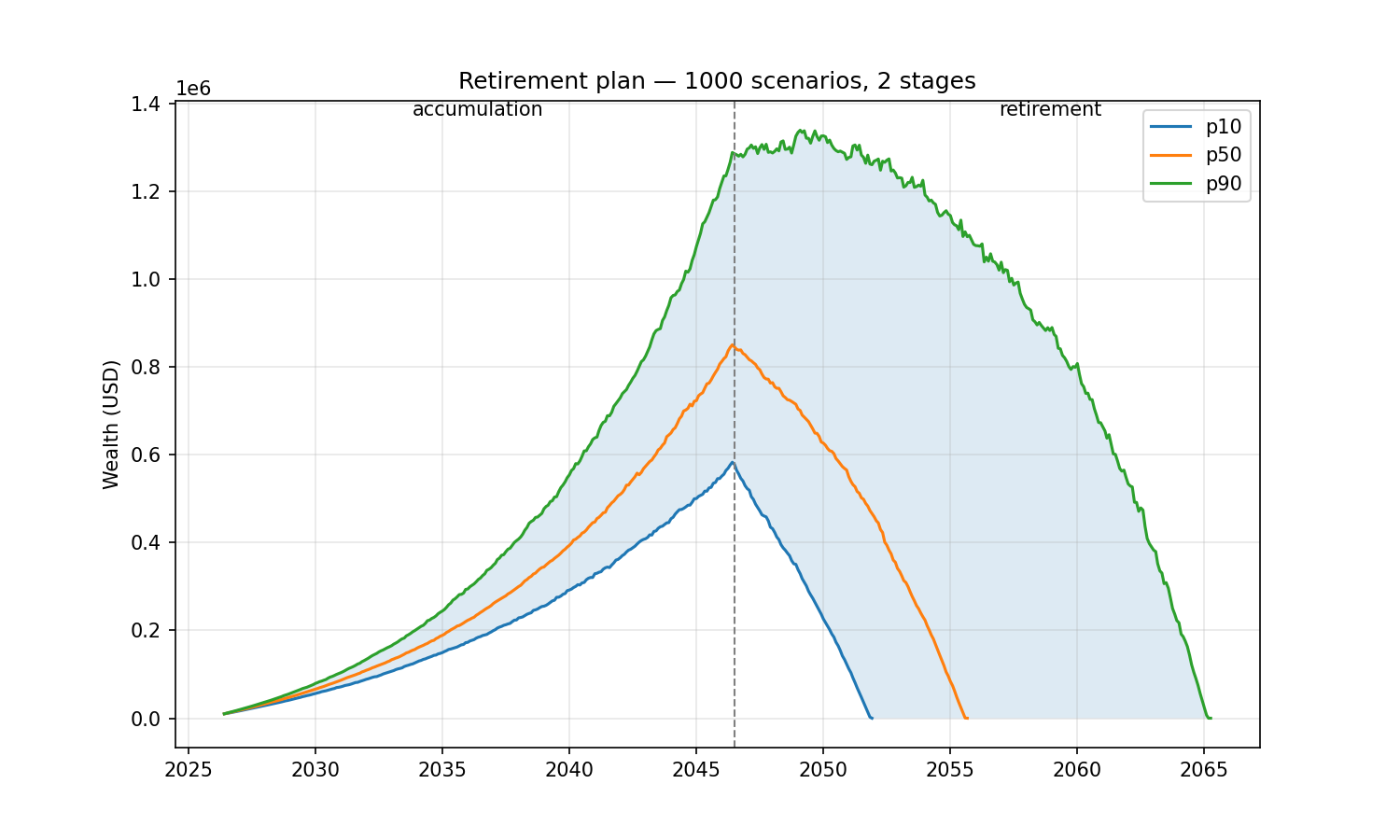
A multi-stage financial plan (contribute $1,000/month for 20 years into a 70/30
SPY/AGG portfolio, then withdraw $6,000/month indexed to inflation for 25 years),
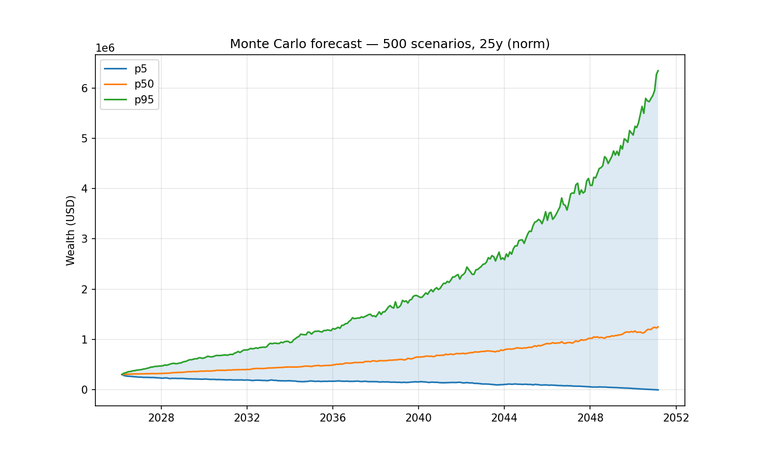
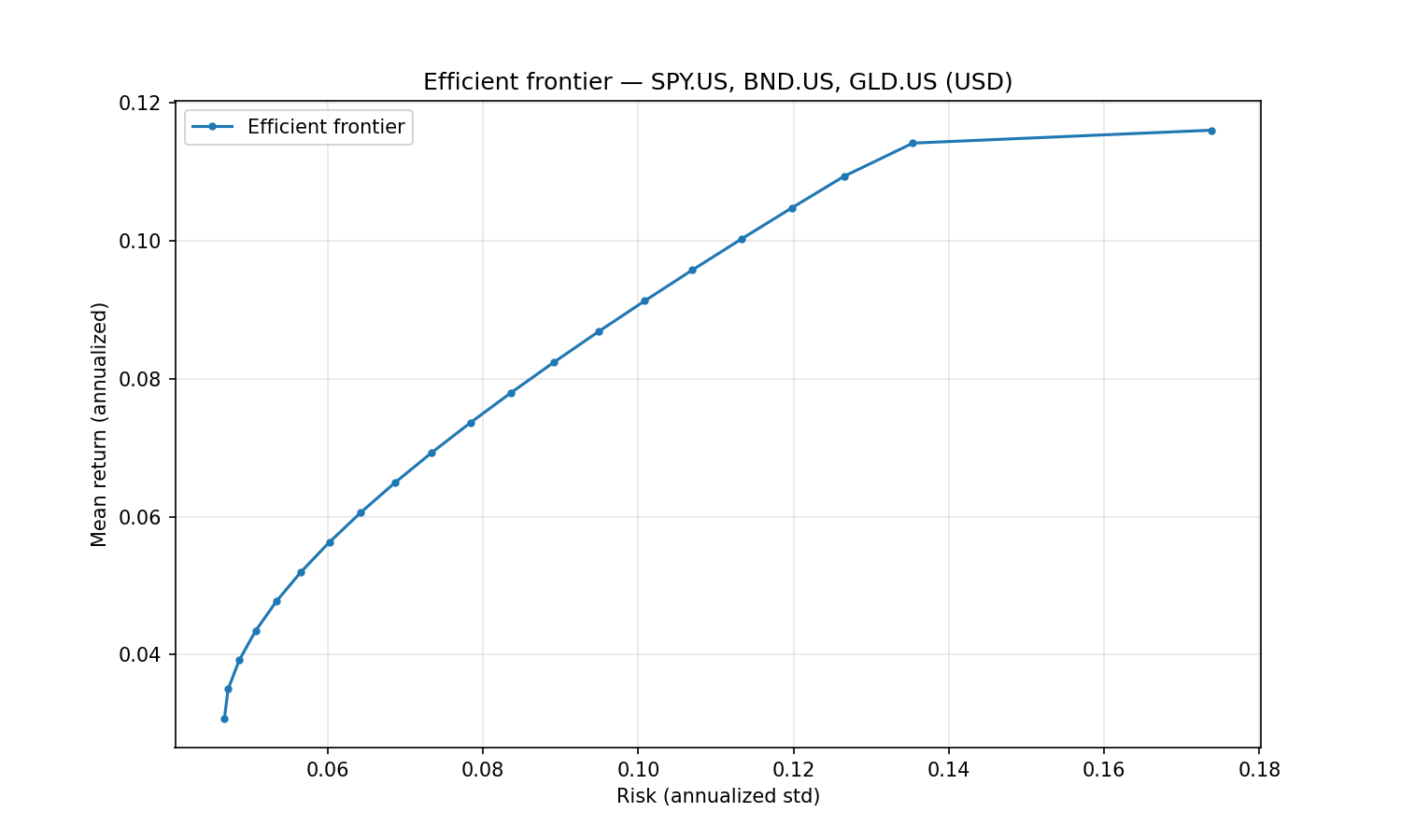
a Monte Carlo retirement forecast (30% gold / 70% real estate, withdrawing $1,000/month
indexed to inflation over 25 years) and the efficient frontier of SPY/BND/GLD:
All tools are **stateless** — pass the full portfolio specification with every call.
The server caches expensive okama objects (`Portfolio`, `EfficientFrontier`) by content
hash, so repeated calls on the same spec are fast.
**Nested portfolios.** Wherever a list of assets is accepted — the `assets` field of
`PortfolioSpec`/`FrontierSpec`, or the `portfolios` argument on the comparison tools —
an entry may be a ticker string **or a nested portfolio object** (the same spec shape).
This lets you treat a whole portfolio as a single component: e.g. compare a 60/40
portfolio against gold, or put a sub-portfolio on the efficient frontier.
### Search & metadata
| Tool | Purpose |
|---|---|
| `search_assets(query="", namespace?, asset_type?, oldest_first?, limit=50)` | Free-text search by name / local name / ticker / ISIN. Filter by okama type and sort by `first_date`; for example, `namespace="MOEX", asset_type="ETF", oldest_first=true, limit=5` finds the five oldest MOEX-listed BPIFs. |
| `list_namespaces(kind="all"\|"assets"\|"macro")` | Show the available okama namespaces. |
| `get_asset_info(symbol)` | Metadata for one symbol — name, country, currency, type, date range. |
### Single asset & comparisons
| Tool | Purpose |
|---|---|
| `get_asset_history(symbol, kind, first_date?, last_date?)` | Time series for one asset. `kind` ∈ {`close_monthly`, `close_daily`, `adj_close`, `ror`, `dividends`}. |
| `compare_assets(symbols, ccy, ..., portfolios?, rf_return?, t_return?)` | Side-by-side statistics (`describe()` table: CAGR, risk, drawdowns by period) plus Sharpe & Sortino per asset. |
| `get_correlations(symbols, ccy, ..., portfolios?)` | Correlation matrix of monthly returns. |
| `get_rolling_risk(symbols, ccy, window_months=12, ..., portfolios?)` | Rolling annualized risk per asset. |
| `get_asset_returns(symbols, ccy, ..., portfolios?, period?, real=False)` | Return metrics per asset: CAGR, cumulative return, mean / real mean return, monthly geometric mean, annual returns table. |
| `get_rolling_returns(symbols, ccy, window_months=12, real=False, ..., portfolios?)` | Rolling CAGR and rolling cumulative return per asset. |
| `get_benchmark_metrics(benchmark, symbols, ccy, ..., portfolios?, rolling_window?)` | Beta, correlation, annualized tracking difference and tracking error of each asset vs a benchmark/index. |
| `get_dividend_info(symbols, ccy, ...)` | LTM dividend yield, 5y mean yield, paying/growing streaks per asset. |
### Portfolio backtest
| Tool | Purpose |
|---|---|
| `analyze_portfolio(portfolio, rf_return=0, t_return=0)` | Headline metrics (CAGR, annual mean/risk, **Sharpe, Sortino**) + full `describe()` for a `PortfolioSpec`. |
| `get_portfolio_drawdowns(portfolio)` | Drawdown time series + max drawdown / recovery period. |
| `get_portfolio_var_cvar(portfolio, time_frame=12, level=1)` | Historical Value at Risk and CVaR. |
| `get_portfolio_wealth_index(portfolio, full=False)` | Wealth-index series (cumulative growth of 1000). |
| `get_rolling_cagr(portfolio, window_months=12, real=False)` | Rolling CAGR time series (optionally inflation-adjusted). |
| `get_cagr_probability(portfolio, years, cagr_target)` | Historical probability of CAGR below a target (e.g. of a loss) over N-year periods. |
### Monte Carlo DCF
| Tool | Purpose |
|---|---|
| `monte_carlo_forecast(portfolio, mc, cashflow)` | Forward simulation with one of five cash-flow strategies (`indexation`, `percentage`, `time_series`, `vanguard`, `cut_if_drawdown`). Returns percentile wealth bands, terminal-wealth stats, survival metrics. Includes the money-weighted IRR distribution (percentiles + mean). |
| `get_portfolio_irr(portfolio, cashflow)` | Historical money-weighted return (IRR) for a contribution/withdrawal plan. |
| `find_the_largest_withdrawals_size(portfolio, mc, cashflow, goal, ...)` | Largest sustainable withdrawal (Monte Carlo) for a `goal`: keep real purchasing power, keep nominal balance, or survive N years. |
| `get_monte_carlo_cash_flow(portfolio, mc, cashflow, discounting?)` | Monte Carlo distribution of future cash flows over time (percentile bands). |
The `mc` argument accepts `distribution_parameters` to override the fitted distribution (e.g. a fixed Student-t `df`); see the MCSpec shape below.
### Financial plan (multi-stage)
A plan is an ordered sequence of stages, each with its own portfolio, horizon and
cash-flow regime. Scenarios are chained: the balance a Monte Carlo scenario ends a
stage with is the balance it starts the next one with, so the retirement stage is
funded by whatever the accumulation stage produced **in that same scenario** — not by
a percentile of it. Use these instead of `monte_carlo_forecast` whenever the portfolio
or the contribution/withdrawal regime changes partway through the horizon.
| Tool | Purpose |
|---|---|
| `finplan_forecast(plan, success_threshold=0)` | Monte Carlo forecast of the whole plan: percentile wealth bands, terminal-wealth stats, survival metrics, the share of scenarios finishing above `success_threshold`, the balance distribution at every stage boundary, and the IRR distribution. |
| `finplan_backtest(plan, discounting?, first_date?)` | Replay the same plan over real history — a glide-path backtest. Requires the window covered by every stage portfolio to be at least as long as the plan. |
### Distribution diagnostics
| Tool | Purpose |
|---|---|
| `get_distribution_fit(portfolio, mc)` | Goodness-of-fit for the return distribution: fitted parameters, Jarque-Bera, Kolmogorov-Smirnov (chosen + all distributions), and backtesting error (theoretical vs empirical mean/VaR/CVaR). |
| `get_return_moments(portfolio, mc, rolling_window?)` | Skewness & kurtosis time series — expanding, or rolling when a window (months) is given. |
| `optimize_students_df(portfolio, mc, var_level?)` | Degrees of freedom for a Student-t that best matches empirical VaR/CVaR. |
| `get_cagr_distribution(portfolio, mc, percentiles?, score?)` | Simulated CAGR at each percentile, plus the probability of a CAGR at/below `score` (e.g. `score=0` → probability of a loss). |
### DCF (historical cash-flow analysis)
| Tool | Purpose |
|---|---|
| `get_dcf_wealth_index(portfolio, cashflow, discounting?, include_negative_values?, discount_rate?)` | Historical wealth index with the cash-flow plan (FV nominal or PV discounted). |
| `get_dcf_cash_flow_ts(portfolio, cashflow, discounting?, remove_if_wealth_index_negative?, discount_rate?)` | Historical contribution/withdrawal time series (FV or PV). |
| `get_dcf_wealth_with_assets(portfolio, cashflow)` | Historical wealth index for the portfolio and each underlying asset. |
| `get_survival_period(portfolio, cashflow, threshold?, discount_rate?)` | Historical longevity: survival period (years) and depletion date. |
| `get_initial_investment_values(portfolio, cashflow, discount_rate?)` | Present value (PV) and future value (FV) of the initial investment. |
### Efficient Frontier
| Tool | Purpose |
|---|---|
| `build_efficient_frontier(frontier)` | Full EF point table (Risk / Mean return / CAGR + per-asset weights). |
| `get_tangency_portfolio(frontier, rf_return, rate_of_return)` | Max-Sharpe portfolio on the EF. |
| `get_min_variance_portfolio(frontier)` | Global Minimum Variance portfolio. |
| `get_most_diversified_portfolio(frontier, target_return?)` | Most Diversified Portfolio (maximises the diversification ratio) on the EF. |
### Macro
| Tool | Purpose |
|---|---|
| `get_inflation(currency, first_date?, last_date?, include_cumulative?, include_rolling?, include_describe?)` | Inflation series for a currency (`USD`, `EUR`, `RUB`, …). Optional: cumulative inflation, 12-month rolling inflation, describe() table. |
| `get_central_bank_rate(country, first_date?, last_date?, frequency="monthly"\|"daily", include_describe?)` | Central-bank policy rate (`US`→US_EFFR, `EU`/`ECB`→EU_MRO, `RUS`→RUS_CBR, `UK`/`GB`→UK_BR, `ISR`→ISR_IR, `CN`/`CHN`→CHN_LPR1, or full symbol). Monthly or daily series; optional describe() table. |
| `get_indicator(symbol, first_date?, last_date?, include_describe?)` | Macro indicator from the RATIO namespace (e.g. `USA_CAPE10.RATIO`); bare country code defaults to that country's CAPE10. |
### Charts
Each tool renders a PNG (default 1500×900) and returns it as MCP image content —
clients like Claude Desktop display it inline. Every chart tool also accepts
optional `width` / `height` (pixels, 300–4000) for custom sizes and aspect ratios,
and an optional `save_path` — the chart is then also written to that file and the
path reported back. Use `save_path` in clients that don't render MCP images in
their UI (e.g. Claude Code's terminal): ask for a chart "saved to /tmp/chart.png"
and open the file reference. Note: in self-hosted (streamable-http) deployments
`save_path` is written on the **server's** filesystem, not the client's machine.
| Tool | Chart |
|---|---|
| `plot_wealth_index(portfolio)` | Portfolio wealth index (+ inflation line). |
| `plot_drawdowns(portfolio)` | Drawdown depth over time. |
| `plot_monte_carlo(portfolio, mc, cashflow)` | Monte Carlo forecast fan (percentile bands). |
| `plot_finplan_forecast(plan)` | Financial-plan forecast fan: percentile bands with dashed stage boundaries and stage labels. |
| `plot_irr_distribution(portfolio, mc, cashflow)` | Histogram of IRR across Monte Carlo scenarios (percentile markers). |
| `plot_qq(portfolio, mc)` | Q-Q plot of historical returns against the fitted distribution (norm/lognorm/t). |
| `plot_hist_fit(portfolio, mc, bins?)` | Histogram of historical returns with the fitted distribution PDF overlaid. |
| `plot_efficient_frontier(frontier)` | EF curve with individual asset points. |
| `plot_transition_map(frontier, x_axe="risk")` | Transition map: asset weights along the efficient frontier (x-axis = risk or CAGR). |
| `plot_assets(symbols, ccy, ..., portfolios?)` | Wealth-index comparison of individual assets. |
| `plot_macro(symbols, first_date?, last_date?, frequency="monthly"\|"daily")` | Line chart of inflation / central-bank rate / CAPE10 series. Overlay multiple symbols (e.g. `["USA_CAPE10.RATIO", "EUR_CAPE10.RATIO"]`). `frequency='daily'` valid only for `.RATE` symbols. |
## Spec shapes
The complex tools take typed dicts validated by pydantic. The full schemas live in
`src/okama_mcp/schemas.py`; here are the headline shapes:
```jsonc
// PortfolioSpec
{
"assets": ["GLD.US", "VNQ.US"], // each entry: a ticker OR a nested PortfolioSpec
"weights": [0.3, 0.7], // optional, must sum to 1.0
"ccy": "USD",
"first_date": "2010-01",
"last_date": "2024-12",
"rebalancing_strategy": { // mirrors okama.Rebalance
"period": "year", // month | quarter | half-year | year | none
"abs_deviation": 0.05, // optional, |actual - target| threshold, 0 < x <= 1
"rel_deviation": 0.1 // optional, |actual / target - 1| threshold, > 0
},
"inflation": true
}
// MCSpec
{
"distribution": "norm", // norm | lognorm | t
"period_years": 25,
"scenarios": 500, // ≥ 1, no upper limit
"percentiles": [5, 50, 95],
"random_seed": 42, // optional, for reproducibility
"distribution_parameters": null // optional; null = fit from history (MLE). Lengths: norm [mu, sigma]; lognorm/t [shape|df, loc, scale]. Any element null = fit that one (e.g. [4, null, null])
}
// CashflowSpec — discriminated by `type`
{ "type": "indexation", "initial_investment": 1000000, "frequency": "month", "amount": -1000, "indexation": "inflation" }
{ "type": "percentage", "initial_investment": 1000000, "frequency": "year", "percentage": -0.04 }
{ "type": "time_series", "initial_investment": 100000, "events": { "2030-06": -50000 }, "time_series_discounted_values": false }
{ "type": "vanguard", "initial_investment": 1000000, "percentage": -0.04, "floor_ceiling": [-0.025, 0.05], "indexation": "inflation" }
{ "type": "cut_if_drawdown", "initial_investment": 1000000, "frequency": "year", "amount": -60000, "indexation": "inflation",
"crash_threshold_reduction": [[0.2, 0.4], [0.5, 1.0]] }
// FinPlanSpec — a plan is a sequence of stages, chained per scenario
{
"stages": [
{ "portfolio": { "assets": ["SPY.US", "AGG.US"], "weights": [0.7, 0.3] },
"period_years": 20, "name": "accumulation",
"cashflow": { "type": "indexation", "initial_investment": 100000, "frequency": "year", "amount": 12000, "indexation": 0.03 } },
{ "portfolio": { "assets": ["SPY.US", "AGG.US"], "weights": [0.3, 0.7] },
"period_years": 25, "name": "retirement",
"distribution": "t", "distribution_parameters": [5, null, null],
"cashflow": { "type": "percentage", "initial_investment": 100000, "frequency": "year", "percentage": -0.04 } }
],
"initial_investment": 100000, // balance the first stage starts with
"discount_rate": null, // optional; null lets okama use inflation
"scenarios": 500,
"random_seed": 42, // optional
"percentiles": [10, 50, 90],
"name": "retirement plan"
}
// FrontierSpec
{
"assets": ["SPY.US", "BND.US", "GLD.US"],
"ccy": "USD",
"bounds": [[0.0, 0.7], [0.1, 1.0], [0.0, 0.3]], // optional
"n_points": 20,
"rebalancing_strategy": { "period": "year" },
"inflation": false
}
// Nesting — a portfolio used as a single component (works in PortfolioSpec /
// FrontierSpec `assets`, and the `portfolios` argument of the comparison tools):
{
"assets": [
"GLD.US",
{ "assets": ["SPY.US", "AGG.US"], "weights": [0.6, 0.4], "symbol": "bench6040.PF" }
],
"weights": [0.3, 0.7] // one weight per top-level entry
}
```
## Development
The project follows TDD (see `AGENTS.md`). After every code change run:
```bash
poetry run pytest -q
poetry run ruff check .
```
To run the live-API integration test (hits `api.okama.io`):
```bash
poetry run pytest -m integration
```
## Project layout
```
src/okama_mcp/
├── server.py # FastMCP instance + registration entry point
├── transport.py # CLI: `okama-mcp stdio | http`
├── schemas.py # PortfolioSpec, MCSpec, CashflowSpec, FrontierSpec, FinPlanSpec
├── cache.py # TTL+LRU cache keyed by sha256 of canonical spec
├── serialization.py # pandas → JSON-safe with smart truncation
├── errors.py # Translate okama exceptions to actionable MCP errors
└── tools/
├── search.py, asset.py, asset_list.py
├── portfolio.py, monte_carlo.py, finplan.py
├── frontier.py, macro.py
└── plots.py
```
## License
[MIT](LICENSE) — same license as okama itself.